The extreme tail of Collatz stopping times is thinner than the Lagarias–Weiss random walk by a factor set by the odd-step ratio, a cliff of 2.1 decades over 0.008 in the ratio
The question
Write T(n) = n/2 for even n and (3n+1)/2 for odd n, let σ_T(n) be the number of T-steps from n to 1, and let γ(n) = σ_T(n)/ln n. A typical n has γ ≈ 6.952; the largest known value is 36.72, at n ≈ 7.2 × 10²¹. In 1992 Lagarias and Weiss modelled the orbit of n as a random walk on ln n with equiprobable steps +ln(3/2) and −ln 2, stopped when it first reaches 0, and proved that in that model lim sup γ(n) = 41.677647…, attained by orbits whose fraction of odd steps is 0.609. Kontorovich and Lagarias (2009) conjecture the same limsup for the integers, and remark that the model's finite-x count of integers with γ ≥ g is "well-suited for comparison with experimental data". That comparison had not been made. This project makes it: the model's predictions are computed exactly at finite x, with no asymptotic exponent and no o(1), and set against every integer below 10¹², the confirmed stopping-time records to 4.66 × 10¹⁹, and every known integer of large γ beyond that, out to 3.8 × 10³¹.
What was known
- Lagarias and Weiss (1992) tabulated the maximum of γ per decade to 10¹¹ and remarked on "a possible leveling off around a value of 32, which is somewhat less than Conjecture 1 predicts". They judged this an end effect of small numbers, consistent with 41.68, because the extremal trajectories show an initial rise and a final plunge that the asymptotic shape does not. Their Section 6 analyses Vyssotsky's greedy backward search and finds that a search of depth 800 attains γ = 30.0 and depth 1000 attains 31.6.
- Applegate and Lagarias (2003) searched the tree of preimages to depth 60 and found no path of odd ratio ½ where the branching model expects hundreds, which they called surprising. The same paper says the stochastic models expect "about 32" below 10¹⁷; read against the 1992 original that is the greedy constant at depth 800–1000, and no finite-x expectation of the record was ever evaluated (the model's actual expected record is 41.46 at 1.05 × 10¹⁷).
- Kontorovich and Lagarias (2009, Table 1) list γ records to 7.2 × 10²¹, the last four marked unverified, and compare them only with the limiting constant.
- Eric Roosendaal maintains the list of 149 confirmed delay records, the largest 46,645,791,847,966,786,687 ≈ 4.66 × 10¹⁹, with every smaller integer checked. His completeness page argues informally, from class records to delay 8000, that γ seems bounded "roughly somewhere between 35 and 45" and that values near 41.68 have not been seen; it also carries Farin's derivation of 0.6090897 as the odd ratio at which the counting heuristic runs out.
- Rozier (2017) conjectures a lower bound on the minimum of a parity class; his own Theorem 2.6 shows it holds trivially below odd ratio 0.609, so it constrains nothing in the range measured here.
- Tao (2019) proved that almost all orbits reach almost bounded values. ProofAtlas published a complete Lean 4 formalization in 2026; an audit of its imports (Appendix A of the repository README) finds nothing beyond finite Fourier analysis on Z/3ⁿ, discrete probability and one harmonic-sum integral.
- Barina's verification to 2⁷¹ ≈ 2.4 × 10²¹ publishes path records only, so the γ-record sequence above 4.66 × 10¹⁹ cannot be recovered from it.
What we did
The unit of comparison is a cell. Group integers by (k, a) with k = σ_T(n) and a = the number of odd steps on the orbit. Up to a residue factor that lies in [1, 1.2532), ln n = k ln 2 − a ln 3, so each cell is a finite population in the data and a finite expected count in the model, and the ratio R(k, a) = integers ÷ model expectation has no x in it. Two coordinates on a cell are used throughout: the excess a − k/2 and the odd ratio r = a/k. Since γ = 1/(ln 2 − r ln 3) up to the residue, fixing γ is nearly the same as fixing r, and the limsup of γ is the supremum of attainable r: 41.68 corresponds to r = 0.6091, 36.2 to r = 0.6057, and one unit of γ near 36 is 0.0007 in r.
The census. Four C programs memoise (σ_T, odd steps) for n < 2²⁸ and iterate above, covering n < 10⁹ in 20–60 s on 2 cores. src/joint12.c extends this to n < 10¹² in one pass: a 2³² memo of (σ_T, ones) packed into 32 bits (16 GB) and 128-bit iteration above it, because orbits that start below 10¹² peak above 2⁶⁴. The recorded run took 16,093 s wall (4.5 h) on 32 cores, part of it throttled to 8. Three checks: the n < 10⁹ column agrees with the earlier census on every cell; the 89 delay records under the Collatz map below 10¹² are identical to Roosendaal's confirmed list; and below 10¹² the records under σ_T and under σ_C are the same 89 integers. Separately, verify/ is a Rust reimplementation of the cell census written from the definitions without reading the C source, with overflow-checked arithmetic; compared cell by cell against the C output at the 10⁹, 10¹⁰ and 10¹¹ cutoffs it has zero mismatches.
The model. src/lwmodel.c computes the walk's survival probabilities by dynamic programming in the log domain, and scripts/analyze_tail.py integrates them to get the expected number N(x, γ) of n ≤ x with γ(n) ≥ γ, all polynomial prefactors kept. src/lwjoint.c resolves the same model by cell; its total over cells reproduces x to 0.7%. The model also has a closed form per parity pattern: for a pattern with odd steps at given positions the walk's weight is 3⁻ᵃ(1 − max(½, 3·max_m t_m))₊ with t_m = 3^(a−1−m) 2^(i_m − k), and summing it over patterns reproduces lwjoint's cell masses to 3% from 40,000 samples. verify/walk_check.py recomputes the committed model table from that closed form with nothing of lwjoint's dynamic programme reused.
Comparison. A cell is complete below x when the walk puts ≥ 99.5% of its mass there; there are 3,215 such cells below 10⁹ and 7,325 below 10¹², with the excess reaching 83 and ln n running from 8 to 28. Counts are pooled within a bin as log(Σ observed / Σ model) with the Poisson error 1/√Σ observed, and fits use log((h + ½)/m) with weight min(m, 10⁴) so that the bulk cells do not own the fit. Neighbouring cells are not independent (the twelve delay records that share the orbit of 63,728,127 are twelve cells' worth of one event), so errors are cluster-robust over 80 × 40 blocks in (k, a), which makes them 3–7 times larger than the naive ones.
Records and far integers. scripts/analyze_records.py recomputes σ_T and the odd count for each of Roosendaal's 149 records by direct iteration and takes the running maximum of γ. Nine integers above 4.66 × 10¹⁹ with large γ are known, from Kontorovich–Lagarias, Roosendaal's strength-record candidates and Vyssotsky's 1997 integer; all nine come from backward searches that select for large γ or strength, and orbits that merge above 10⁶ are grouped into five families.
Decomposition. scripts/explore_geometry.py samples 40,000 parity patterns per cell for seventeen cells along the ridge and splits R into the part the walk's geometry explains and a residual arithmetic factor D. src/digits.c samples 10⁹ first-passage patterns per cell (about 25 min on 32 cores) and records how often 3^j divides 2^k − r_v for j ≤ 12 among patterns that obey the residue bound. src/tails.c records the full parity pattern of every integer in twelve cells complete below 10⁹ (93,700 patterns) for comparison with uniformly random admissible patterns. src/joint_3nm1.c runs the same census for the 3n−1 map, which is the 3n+1 map on the negative integers, to 10¹¹ (21 minutes on 32 cores). scripts/tao_tilt.py computes the exact Syracuse distributions mod 3ⁿ for n ≤ 12 under a tilted valuation law (1 s) and reproduces Tao's listed Syrac(Z/9) probabilities exactly.
What we found
Bulk agreement, tail deficit. The model matches the number of n ≤ 10⁹ with γ(n) ≥ γ to within 4% for γ ≤ 8 and 10% at γ = 9. Beyond that the integers fall below it: at x = 10⁹ the observed/expected ratio is 0.53 at γ = 13, 0.18 at γ = 20, 0.10 at γ = 30 and 0.025 at γ = 32. At the actual record below 10⁹, γ = 32.94, the model expects about 44 integers and there is one.
The variable is the odd ratio. On the 2,914 cells with ≥ 20 integers complete below 10⁹ the deficit looked like a function of the excess, R ≈ 1.2 · 0.954^excess. The census to 10¹² shows that was a projection: within the 10⁹ strip the excess and ln n are nearly collinear, and at fixed excess R rises with ln n, the slope in the excess falling from 0.11 per step at ln n ≈ 14 to 0.03 at ln n ≈ 26. The variable on which the ln n bands collapse is r. Pooled over all complete cells, binned in r and ln n, with log(Σ observed / Σ model) ± its Poisson error and the number of cells in brackets:
| r | ln n 8–14 | 14–18 | 18–22 | 22–25 | 25–28.5 |
|---|---|---|---|---|---|
| 0.550–0.555 | +0.07 ± 0.01 (40) | −0.02 (44) | −0.07 (53) | −0.09 (49) | −0.10 (47) |
| 0.560–0.565 | −0.25 ± 0.01 (46) | −0.29 (57) | −0.31 (72) | −0.31 (62) | −0.31 (64) |
| 0.570–0.575 | −0.78 ± 0.02 (44) | −0.75 (78) | −0.69 (97) | −0.63 (85) | −0.59 (84) |
| 0.580–0.585 | −2.06 ± 0.08 (27) | −1.44 ± 0.01 (113) | −1.07 (142) | −1.00 (126) | −0.95 (123) |
| 0.590–0.595 | −2.21 ± 0.06 (49) | −1.81 ± 0.01 (221) | −1.58 (198) | −1.33 (196) | |
| 0.595–0.600 | −2.28 ± 0.05 (65) | −1.44 ± 0.01 (188) | −1.60 ± 0.01 (249) | ||
| 0.600–0.605 | −2.59 ± 0.14 (18) |
On the shoulder (r ≤ 0.575) the bands agree to ±0.1 over a factor e¹⁸ in n. On the steep part they fan out by about a nat, from −2.06 at ln n 8–14 to −0.95 at 25–28.5 for r = 0.580–0.585, with larger n less suppressed. Measured as ∂ log R/∂ ln n at fixed r with cluster-robust errors, the drift is +0.006 ± 0.003 per nat on the shoulder (r 0.55–0.58), +0.034 ± 0.005 on the steep part (0.58–0.605) and +0.086 ± 0.007 at r ≥ 0.59. The sign matters for what comes later: a law in the excess would require R to fall with n at fixed r, because the excess k(r − ½) grows with n.
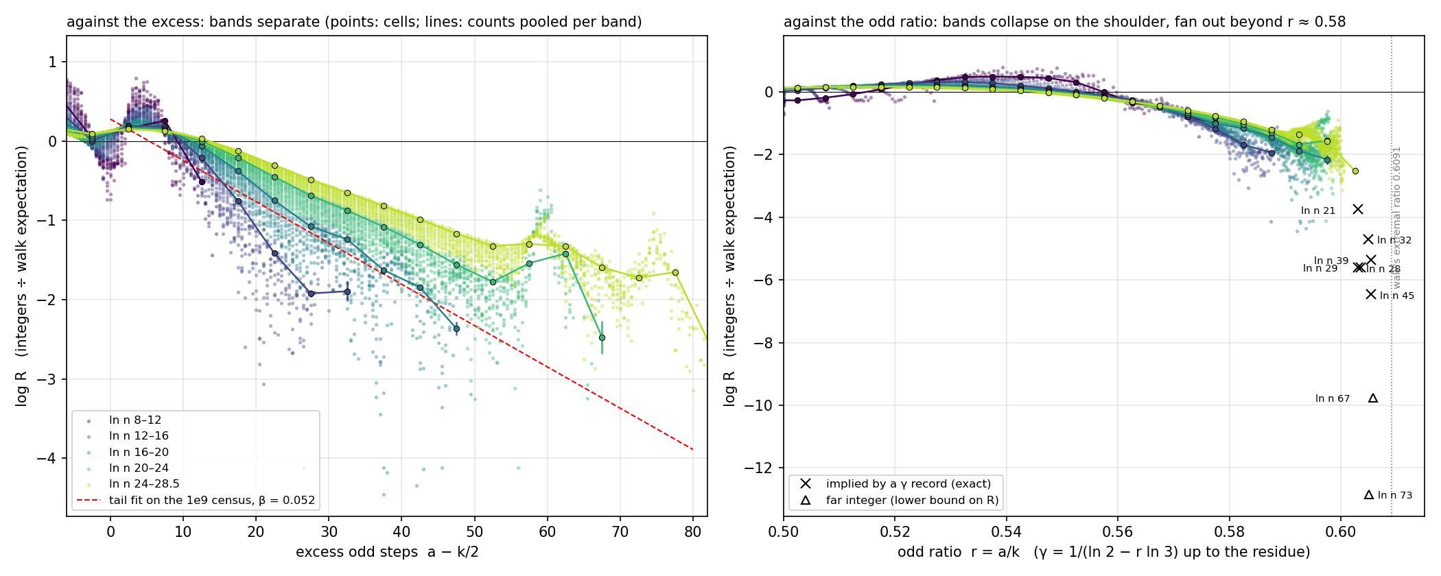
The records continue the cliff. A γ record at n with nothing larger below x says the cells with γ ≥ that record hold one integer where the walk expects N_RW(x, γ), so their average R is 1/N_RW. That gives 10⁻¹·⁶ at r = 0.603 (x = 10⁹), 10⁻²·⁴ when the same record still stands at 10¹², 10⁻²·⁴ at r = 0.6035 (n = 3.7 × 10¹²), 10⁻²·⁰ at 0.6049 (10¹⁴), 10⁻²·³ at 0.6054 (1.05 × 10¹⁷) and 10⁻²·⁸ at 0.6054 by the verified limit 4.66 × 10¹⁹. Each is read off a single extreme value: the expected count at the realised maximum is Exp(1)-distributed, so log(1/N_RW) estimates log R with a bias of +0.58 and a standard deviation of 1.3 nats (0.56 decades), and neither the ordering of these six values along r nor the drop from 10⁻¹·⁶ to 10⁻²·⁴ between 10⁹ and 10¹² is outside that noise. What is supported is the fall from 10⁻⁰·⁷ at r ≈ 0.5975 (cells) to 10⁻²·⁸ at r = 0.6054 (the last record, complete data): 2.1 decades over 0.008 in r, a slope of 0.27 decades per 0.001. Beyond 0.6054 nothing in the data bounds R from above. The far integers each put at least one integer where the walk expects N_RW, so they bound R from below: R ≥ 10⁻⁴·² at r = 0.6057 (1.8 × 10²⁹) and R ≥ 10⁻⁵·⁶ at 0.6051 (3.8 × 10³¹). The lower bound at 0.6057 caps the mean cliff slope beyond the cells at 0.4–0.6 decades per 0.001.
The model fails the record test. Laws fitted on cells below 10⁹ were tested on the four confirmed records above it. Expected number of integers n ≤ x with γ(n) ≥ the confirmed record at x (observed: exactly one in each row):
| x | record | random walk | linear 0.052 | linear 0.047 | linear + ln n | sublinear |
|---|---|---|---|---|---|---|
| 3.74 × 10¹² | 33.37 | 269 | 5.1 | 6.8 | 3.5 | 8.9 |
| 1.01 × 10¹⁴ | 35.17 | 111 | 1.6 | 2.1 | 0.92 | 2.9 |
| 1.05 × 10¹⁷ | 35.82 | 210 | 1.2 | 1.6 | 0.71 | 2.6 |
| 4.66 × 10¹⁹ | 35.82 | 641 | 1.3 | 1.8 | 0.89 | 3.9 |
The random walk expects 641 integers at or above the record 35.8238 below 4.66 × 10¹⁹, 132 at or above 37, 37 at or above 38 and 3.8 at or above 40; the probability of the observed outcome under it is e⁻⁶⁴¹ ≈ 10⁻²⁷⁸. Its predicted record at 4.66 × 10¹⁹ is 41.6 against the observed 35.82. The suppressed laws expect of order one integer at the last three points; at the first point the linear laws expect 5.1 and 6.8 where one was observed (P(≤ 1) = 0.037 and 0.009), which on the ±1.3-nat scale of a single extreme value is a 2–2.6σ miss. The far integers push the other way: under the linear laws the far ranges are nearly empty (expected 0.02–0.4 per family for families 1–4), and the joint probability of at least one integer in each family's range is 6 × 10⁻⁶ (β = 0.052) or 3 × 10⁻⁴ (β = 0.047), against 0.12 for the sublinear law. No law in the one-variable excess family fits comfortably; the r × ln n table above says why.
What the cliff is made of. Three things it does not depend on. Inside a cell the number of adjacent odd pairs matches the fair-coin baseline to 0.2 on a mean near 100, so the parity vector is a uniformly random arrangement given (k, a) and the deficit is in cell populations. Residue indicators for k mod 2, 3, 4 and a mod 2, 3 are all within ±0.011. And the residuals of neighbouring cells correlate at 0.94–0.97, so the deficit is a coherent function of position.
The walk's weight for a parity pattern is a window condition on n; the exact count is the number of patterns that satisfy both an admissibility condition on the orbit and the congruence 3^a | 2^k − r_v. Splitting R along that line, with positivity of n as the admissibility condition, the walk's geometry accounts for one fifth of the slope in the excess (e^(−0.008·excess) of a total e^(−0.040·excess)) and the congruence for four fifths. Positivity is too weak a condition: the residue product ∏(1 + 1/(3m_i)) never exceeds 1.2532 (Roosendaal's Conjecture 2b, verified to 2³² and by every cell here), which at the pattern level is Σt ≤ 1 − 1/1.2532 = 0.2020, and it says the orbit does not pass through small odd values too early. Under that condition the split is half and half: the geometric factor falls from 0.42 at excess 0 to 0.18 at excess 40 (e^(−0.021·excess)), and the residual arithmetic factor D_res from 2.7 to 1.2 (e^(−0.019·excess)). In the bulk, among dynamically plausible patterns, the congruence is met nearly three times as often as chance, and that advantage is what dense cells lose.
Which 3-adic digits carry the arithmetic half: conditional on the residue bound, the factor D_j = 3^j · P(3^j | 2^k − r_v) by which the congruence mod 3^j beats chance, and its decline from excess 0 to excess 55:
| j | D_j in the bulk cell | decline from excess 0 to 55 |
|---|---|---|
| 1 | 1.67 | 2% |
| 4 | 1.8–2.0 | 6% |
| 5 | 1.8–2.0 | 11% |
| 8 | 1.6–1.8 | 20% |
| 12 | 25% (sampling error ±0.05 to ±0.10) |
Against the full factor D_res, which falls from 2.66 at excess 0 to 1.23 at excess 40.5, about a quarter of the log decline is visible by the eighth digit and no more by the twelfth; three quarters sit above conductor 3¹², in the digits that depend on the whole pattern through carries. The mod-3^j branching model of the backward tree says the same from the other side: at j = 10 (59,049 residue classes) it still overpredicts dense cells by 2× at excess 27.
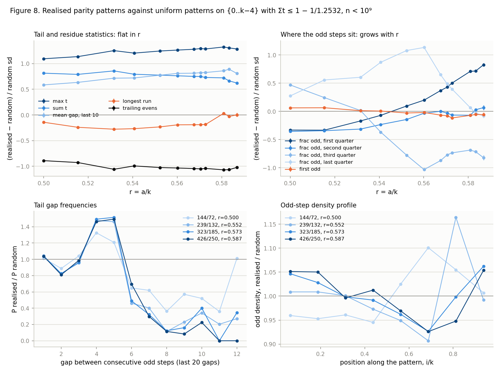
The realised patterns themselves locate the difference. The tail of a real orbit is the orbit of a small odd number and is the same in every cell: the last odd value is 5 in 95–99% of orbits, the last gap is 3 or 5 in 95–98%, and the mean gap over the last ten odd steps is 2.38–2.40 in all twelve cells from r = 0.50 to 0.587. What grows with r is where the odd steps sit along the pattern. Realised patterns at r = 0.50 are back-loaded and at r = 0.587 front-loaded (odd density 1.11, 1.09, 1.03, 1.04, 1.01, 0.94, 0.94, 0.86 by eighth), and the standardised excess of the first-quarter odd share runs linearly from −0.33 at r = 0.50 through zero near 0.545 to +0.83 at 0.587, slope +0.14 per 0.01 in r with standard error 0.01. A heuristic reading is that every suffix of a pattern is itself the orbit of a smaller integer in a cell of its own, so an r-dependent deficit acts on every suffix and pushes odd steps forward where log R falls with r; this is untested against dlog R/dr.
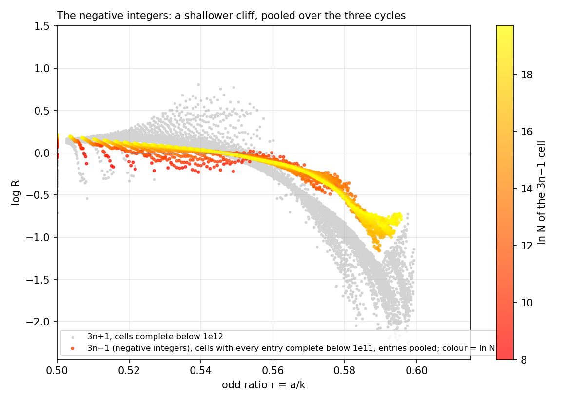
The 3n−1 map. Under 3n+1 the negative integers are the 3n−1 map on the positives, with three cycles entered at eleven elements. Pooling entries with the walk's weight over cells where every entry is complete below 10¹¹ (2,761 cells), the per-cell deficit collapses onto r as on the positive side with about two thirds of the slope (−24.1 ± 1.4 against −36.4 ± 1.2 per unit r, block-bootstrap errors) and about half the depth (−0.72 against −1.3 at r = 0.58–0.59). Per entry it is far from uniform: from the bulk to r = 0.60, orbits reaching the fixed point −1 fall by 2.9 nats against 1.7 on the positive side, while those entering the eleven-cycle at −61 do not fall at all. The levels are measured against the walk's global entry shares, which the r = 0.50–0.51 row shows are the wrong baseline for these cells, so only the trends are meaningful. On the negative integers a large part of the dense orbits the model predicts is redirected into the large cycle; the positive integers have nowhere else to go.
Tao's argument under a tilted valuation law. Tao's Fourier-decay proposition for the Syracuse variable mod 3ⁿ uses, beyond memorylessness and exponential tails of the valuation law, only that the renewal process drifts across the lattice fast enough, which for the tilted law with odd ratio r is the inequality r < 0.6309. The decay survives up to there with continuously degrading constants. The derivation of mixing from the decay is different: it uses that every valuation string of a given total is equiprobable, which is special to r = ½, and for r above 0.6091 the failure is real, because the entropy of the valuation string falls below n ln 3 and the distribution mod 3ⁿ cannot approach uniform. The equation that fixes 0.6091 is H(r) = r ln 3, which is the Lagarias–Weiss limsup equation. Between the census ratios and 0.6091 mixing is neither proved by his argument nor excluded by counting; the cliff occupies exactly the regime in which nothing is known either way.
What it means and what it does not mean
Proved, in the sense of exact computation. The census counts and the record list are exact. The model's finite-x expectations are exact evaluations of the Lagarias–Weiss model with all prefactors, checked by an independent closed form. The statement that the model's finite-x predictions are wrong for the integers below 4.66 × 10¹⁹, at probability 10⁻²⁷⁸, is as firm as those two things.
Measured. The deficit is a function of r alone on the shoulder, and of r and n beyond it, with larger n less suppressed. The cliff slope of 0.27 decades per 0.001 in r between the cells and the last confirmed record is a measurement with the ±1.3-nat uncertainty of a single extreme value at its far end. The half-and-half split between geometry and congruence, the quarter of the congruence part visible by the twelfth 3-adic digit, and the 3n−1 comparison are measurements on sampled patterns and complete cells.
Heuristic. Everything about the limsup. Two readings were on the table. A law in the excess, exp(−β·excess), multiplies the walk's count by a power of x and moves the limsup to 35.8 (β = 0.052) or 36.3 (β = 0.047), near the far integers' flat 36.2–36.7. A suppression F(r) independent of n leaves the limsup at 41.68, because for every r < 0.6091 the walk's count grows like a power of x and any fixed F(r) > 0 is eventually overwhelmed; it ties the finite-x record to the cliff. The census measures the quantity on which the two differ, ∂ log R/∂ ln n at fixed r. The excess law needs −0.11 to −0.13 per nat at r = 0.595; the cells find +0.006 ± 0.003 on the shoulder, +0.034 ± 0.005 on the steep part and +0.086 ± 0.007 at r ≥ 0.59. That excludes the excess law as a law in n and favours the cliff reading. Summing the walk's cells with the cliff as weight, conditional on the confirmed record, the median record is 36.2 at 10²², 36.9 at 10²⁵, 37.6 at 10³⁰, 38.6 at 10⁴⁰ and 39.2 at 10⁵⁰: about 1.7 units of γ per ten orders of magnitude near 10²⁵, 0.9 at 10³⁰–10⁴⁰, 0.6 at 10⁴⁰–10⁵⁰, with γ = 40 near 10⁷⁰. A cliff two or four times as steep lowers these by 0.4–0.9 and barely changes the rate. Within reach of any verification, 2⁷¹ ≈ 10²¹·⁴, the two readings expect the same record to within half a unit of γ; at 10³⁰ they differ by one to two units.
What it cannot do. Carry the measured n-dependence thirty units of ln n beyond the census. At +0.03 to +0.09 per nat that extrapolation is one to three nats, half a decade to a decade, the size of the cliff itself, and whether the drift persists, saturates or reverses above ln n ≈ 30 is untested. A reversal would move the limsup. The record-implied values are too noisy to help and the far integers only bound R from below. A wall near 36–38 stays open on that account.
Whose belief this bears on. Lagarias and Weiss saw the levelling-off near 32 in their 1992 Table 4 and recorded it as an end effect of small numbers; the per-cell comparison controls for the end-game cell by cell, and the plateau is not an end effect. Applegate and Lagarias's "about 32" below 10¹⁷ is their reading of the 1992 greedy-search constant and was never a finite-x expectation, so there is no conflict with the 41.5–41.6 the model actually predicts there. The Kontorovich–Lagarias conjecture that the limsup is 41.68 is favoured by the sign of the n-dependence and is not overturned. Nothing here bears on cycles or on the Collatz conjecture itself; it bears on the model that supplies the constant.
Corrections made in today's referee pass. These are listed so that the checking is visible.
- The far integers were being read in the wrong direction. Each is one integer in a range not searched exhaustively, so it says R ≥ 1/N_RW there, and nothing bounds R from above beyond r = 0.6054. The README now states this at every place the far integers appear, Figure 5 draws them as upward-pointing triangles, and the only quantitative use made of them is the cap of 0.4–0.6 decades per 0.001 on the mean cliff slope beyond the cells.
- The first version of the r × ln n table used only cells with ≥ 20 integers. That cut selects on the dependent variable: a cell whose expected count under the law is below 20 survives it only by fluctuating upward, and bins where no cell survived were blank. It removed exactly the small-n, high-r cells where the deficit is deepest and made the collapse look complete; its deepest kept value was −1.79 against −2.59 now. The table above uses every complete cell. The slope in r is unaffected in substance (−36.4 ± 1.2 on the cut set, −32.9 on all cells) and the n-dependence on the steep part is the new finding the cut had hidden.
- The pattern sampler behind the digit hierarchy admitted patterns with an odd step at k − 2 or k − 3. An orbit first reaching 1 at step k passes 8, 4, 2, so such patterns are never first-passage orbits. The earlier paragraph reported the residue-bound digit factors as flat in the excess to ±0.05 for j ≤ 8; that was wrong on its own numbers (the declines were 7–17% at j = 5–10) and is withdrawn. The same mistake in the geometry split, sampling admissibility on the walk's pattern space, had given D ≈ 0.5 in the bulk, an artefact.
- The admissibility threshold on Σt was rederived. The residue product is bounded by 1.2532, and the condition on patterns that follows is Σt ≤ 1 − 1/1.2532 = 0.2020; the number 0.2532 belongs to the residue, and a threshold on Σt at that value would admit patterns no orbit realises.
- The committed random-walk cell table was recomputed from the per-pattern closed form (
verify/walk_check.py). The two agree on the definition; the committed table carries a discretisation error from lwjoint's trapezoid rule, since the integrand is a step function of ln n whose jumps do not fall on grid points. The error is a few per cent per cell and larger in a column whose cutoff truncates the cell. It is systematic in sign and does not touch the pooled comparison at the scale of the effects above, and a finer grid or an exact sum over the step function would remove it. - An earlier reading of the 3n−1 data as an n-dependence was the entry composition of partially complete cells and is withdrawn; the pooled comparison now uses only cells where all eleven entries are complete.
What is left
The two questions that matter most are a mechanism for the suppression and whether R at fixed r drifts with n beyond ln n = 28, which is the whole difference between a limsup of 41.68 and one near 36. The object for the first is the count of admissible arrangements v with Σ_j 3^(a−1−j) 2^(i_j) ≡ 2^k (mod 3^a); the deviation from 3^(−a) is in the high 3-adic digits, grows with r, and is not in the walk's geometry. A comparison against random patterns additionally conditioned on the low 3-adic digits, which would isolate what lies above the twelfth digit, has not been done, and the suffix heuristic for the front-loading has not been tested against dlog R/dr.
For the second, the next data are delay records. Conditional on the exhaustive data, the expected number of new integers in (4.66 × 10¹⁹, 2⁷¹] with γ ≥ 35.82 is 688 under the random walk, 0.07 and 0.17 under the linear laws and 1.3 (probability 0.73 of at least one) under the sublinear law. Barina's verification reaches 2⁷¹; if the delay records of that range can be extracted they confirm or refute the 2.7 × 10²⁰ integer as a record and give the complete γ-record sequence two more orders of magnitude out. Deciding the limsup itself needs complete records at 10³⁰ or beyond, where the readings are one to two units of γ apart (37.0–37.6 against 35.8–36.0), or a mechanism.
Two smaller items from the pass. The 3n−1 slope −24.1 was fitted on cells with ≥ 20 integers, the cut the positive side has abandoned; the full-cell fit there remains to be done. And the random-walk cell table should be regenerated with a finer grid or an exact step-function sum, after which the per-cell comparison can be rerun.
Reproduce it
cd /neptune/collatz-tail
make build      # gcc with OpenMP
make census     # n < 1e9: ~2 min on 2 cores, 1.5 GB RAM
make models     # survival table, cell tables to 1e9 and 1e20, mod-3^j branching: ~5 min
make analyze    # python3 with numpy, scipy, matplotlib -> data/results/*.md, figures/*.png
make census12   # n < 1e12 (src/joint12.c): 16 GB RAM; 16,093 s wall on 32 cores (not part of `all`)
make census3nm1 # the 3n-1 map to 1e10; LIMIT=11 writes census_3nm1_k_a_1e11.csv (21 min on 32 cores)
make digits     # conditional 3-adic digit hierarchy, 8 cells x 1e9 patterns, ~25 min on 32 cores
make data/results/rw_cells_to_1e12.csv data/results/rw_cells_to_1e32.csv
make data/results/rw_cells_3nm1.csv data/results/rw_cells_3nm1_1e11.csv
cd scripts && python3 analyze_cells_1e12.py && python3 check_records_1e12.py && python3 plot_fig5.py && python3 analyze_tails.py
cd ../verify && cargo build --release
./target/release/verify census <x> <threads> <memo bits> <out.csv>   # recorded runs: 8 threads, 27 memo bits
python3 compare.py                                                    # against census_k_a_1e12.csv
nice -n 19 python3 walk_check.py                                      # the model table from the closed form
All result files are committed, so make analyze alone regenerates every table and figure from the committed data.